Training A Neural Network
Neural network(NN) has many applications. It has large amount of parameters we can train. Usually we train a NN to minimize loss function and make it perform well on some tasks. In this notebook, we are going to walk through a simple NN that can classify data into binary classes.
# import libraries
import seaborn as sns
import numpy as np
import matplotlib.pyplot as plt
preliminary
A neural network usually has many hidden layers and weights matrix as connection. Each unit must pass through activation function to decide fire or not. $$ H_2 = \sigma (H_1 * W_1) $$ $H_1$ and $H_2$ are hidden layers and $W_1$ is weight matrix and $\sigma$ is activation function. $\sigma$ is applied element-wisely.
There are many choices for activation functions, i.e., Sigmoid: $\sigma(x) = \frac{1}{1+e^{-x}} $
The higher output, the higher probability of being 'activated'.
def sigmoid(x):
    return 1. / (1+np.exp(-x))


# a plot sigmoid function
line = np.linspace(-5, 5, 100)
plt.plot(line, sigmoid(line), '.')
plt.ylim(0, 1)
plt.xlabel("input")
plt.ylabel("output")
plt.title("sigmoid")
plt.show()

Steepest gradient descent:
Usually we go a little step to update weight matrix using gradient: $W_1 = W_1 - \alpha \cdot \frac{d L}{d W_1}$. This update rule is justified by steepest gradient descent.
$W_1$ update using derivative $\frac{d L}{d W_1}$(or gradient):
Firstly, we specify our notations:
$H_1^{(i)(j)}$: $i$ th row $j$ th colume in $H_1$, $I$ rows X $J$ columes in total;
$W_1^{(j)(k)}$: $j$ th row $k$ th colume in $W_1$, $J$ rows X $K$ columes in total;
$H_2^{(i)(k)}$: $i$ th row $k$ th colume in $H_2$, $I$ rows X $K$ columes in total;
Let's start by partial derivative of certain element of $W_1$, say $\frac{\partial L}{\partial W_1^{(j)(k)}}$. According to chain rule:
$$
\frac{\partial L}{\partial W_1^{(j)(k)}} = \frac{\partial H_2}{\partial W_1^{(j)(k)}} \cdot \frac{\partial L}{\partial H_2}
$$
So if $W_1^{(j)(k)}$ is changed, $H_2$ will also change; As $H_2$ has changed, so does $L$. We want to sum up all such changes in $L$, our objective is to minimize it:
$$
\frac{\partial L}{\partial W_1^{(j)(k)}} =
\sum_{i=1}^{I} \frac{\partial H_2^{(i)(k)}}{\partial W_1^{(j)(k)}} \frac{\partial L}{\partial H2^{(i)(k)}} \dots \dots (1)
$$
Notice that those are coefficeints of linear function:
$$
\sum_{j=1}^{J} H_1^{(i)(j)} W_1^{(j)(k)} = H_2^{(i)(k)}
$$
Hence, $\frac{\partial H_2^{(i)(k)}}{\partial W_1^{(j)(k)}} = H_1^{(i)(j)}$. Plug it into equation $(1)$ above:
$$
\frac{\partial L}{\partial W_1^{(j)(k)}} = \sum_{i=1}^{I} H_1^{(i)(j)} \frac{\partial L}{\partial H2^{(i)(k)}}
$$
Here is an illustration:
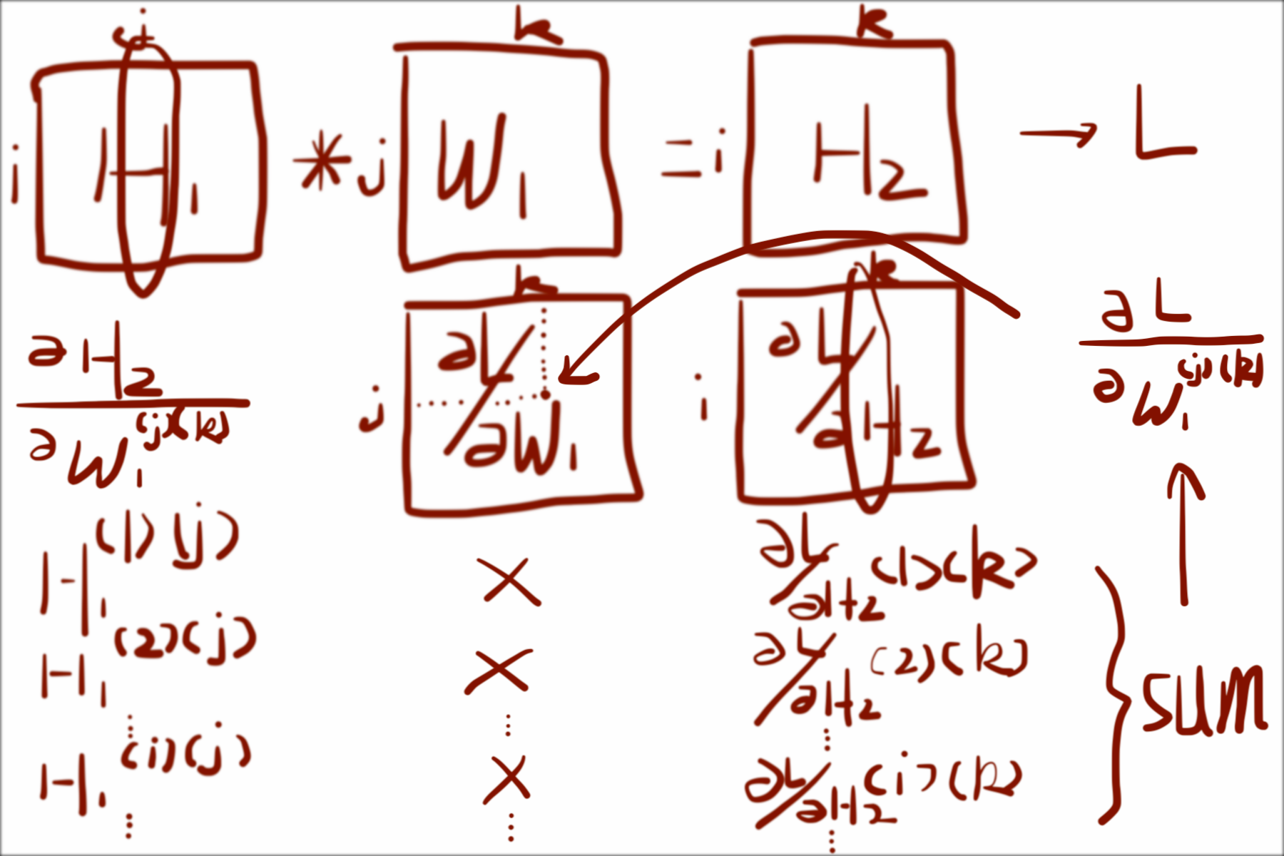
In the image above, $j$ and $k$ is fixed for partial derivative of $W_1^{(j)(k)}$; $\sum$ is over $i$, which can be seen as dot-product between $j$th in $H_1$ and $k$th colume in $\frac{\partial L}{\partial H_2}$.
So far we get $\frac{\partial L}{\partial W_1^{(j)(k)}}$, which is one element in $\frac{\partial L}{\partial W_1}$, but we need the all elements. The interesting thing is that , if we do the same operation to every element using one colume in $H_1$ and one colume in $\frac{\partial L}{\partial H_2}$ and do dot-product, the result is just matrix multiplication between $H_1$ reversed and $\frac{\partial L}{\partial H_2}$:
$$
\frac{\partial L}{\partial W_1} = H_1^T * \frac{\partial L}{\partial H_2}
$$
Where $*$ is matrix multiplication.
Here is an illustration:

You can shift $j$ and $k$ to get any $\frac{\partial L}{\partial W_1^{(j)(k)}}$ of $\frac{\partial L}{\partial W_1}$.
Recall that we want to update our weight matrix $W_1$ using steepest gradient descent: $W_1 = W_1 - \alpha \cdot \frac{d L}{d W_1}$; Now we only need to choose a proper $\alpha$ and train our network!(not really, actually)
Training and Visualization
Step 1: preparing training data.
We are going to train our neural net to do binary classification. So our data consists of 10000 samples from gaussian distribution $g_0\sim N(-6,1)$, and another 10000 samples from $g_1\sim N(6,1)$. We expect our neural net to output probability close to 1 when given new samples from $g_1$ and close to 0 when given samples from $g_0$
# guassian1
g0 = np.random.randn(10000) - 6
g0 = np.expand_dims(g0, 1)
# guassian2
g1 = np.random.randn(10000) + 6
g1 = np.expand_dims(g1, 1)

X = np.vstack([g0, g1])
y = np.vstack([np.zeros_like(g0),\
               np.ones_like(g1)])
# pack data and corresponding label
data_and_label = np.array(list(zip(X, y)))
np.random.shuffle(data_and_label)

X_train = data_and_label[:, 0]
y_train = data_and_label[:, 1]  # true labels

# take a look at firs 5th elements
# in X_train and y_train
print(X_train[:5])
print(y_train[:5])
Step 2: train our neural net!
# define cross-entropy loss function
def binary_logistic_loss(prediction, label):
    y = prediction
    y_hat = label
    epsilon = 1e-4
    error = - y * np.log(y_hat + epsilon) -\
        (1 - y) * np.log(1 - y_hat + epsilon)
    return error
# initialization
Wxh = np.random.randn(1, 32)
bxh = np.zeros(32)
Whh = np.random.randn(32, 1)
bhh = np.zeros(1)

# set step size
step = 1

# train
for i in range(1000):
    # forward:
    h = X_train.dot(Wxh) + bxh
    h_sigmoid = sigmoid(h)
    # hh means h->out
    out = h_sigmoid.dot(Whh) + bhh
    y_hat = sigmoid(out)
    error = binary_logistic_loss(y_hat, y_train)
    L = np.sum(error)/X_train.shape[0]

    # backforward:
    derror = 1./X_train.shape[0]
    # backprop through cross-entropy loss
    dy_hat2error = y_train * 1./(-y_hat) + \
                  (1 - y_train) * (1./(1-y_hat))
    # backpro through sigmoid
    dout2y_hat = (1 - y_hat) * y_hat
    # chain rule
    dout = dout2y_hat * dy_hat2error * derror
    # dW_1 = H_1.T * H_2
    dWhh = h_sigmoid.T.dot(dout)
    dhh = np.sum(dout, 0)
    dh_sigmoid = dout.dot(Whh.T)
    dh2h_sigmoid = (1 - h_sigmoid) * h_sigmoid
    dh = dh2h_sigmoid * dh_sigmoid
    dWxh = X_train.T.dot(dh)
    dbxh = np.sum(dh, 0)

    # update
    Whh -= step * dWhh
    bhh -= step * dhh
    Wxh -= step * dWxh
    bxh -= step * dbxh

    if i % 100 == 0:
        print("epoch: {}; loss: {}".format(i, L))
Step 3: plot result
# X_predict is 10000 real numbers from [-10, 10]
line = np.linspace(-10, 10, 10000)
X_predict = np.expand_dims(line, 1)
# make prediction
h = X_predict.dot(Wxh) + bxh
h_sigmoid = sigmoid(h)
# hh means h->out
out = h_sigmoid.dot(Whh) + bhh
y_hat = sigmoid(out)
# plot
plt.figure(figsize=(6, 6))
sns.distplot(g0, hist=False, kde=True,
             color='darkblue',
             kde_kws={'linewidth': 1})
sns.distplot(g1, hist=False, kde=True,
             color='green',
             kde_kws={'linewidth': 1})

y = np.random.uniform(0, 0.005, size=g0.shape)
plt.scatter(g0, y, marker=".", linewidths=0.0001,\
            alpha=0.05, c='darkblue')
plt.scatter(g1, y, marker=".", linewidths=0.0001,\
            alpha=0.05, c='green')
plt.plot(line, y_hat, color='r')

plt.legend(["Decision Boundary"])
plt.xlabel('x')
plt.ylabel('density')
plt.title('Histogram')
plt.text(60, .025, r'$\mu,\ \sigma$')
plt.axis([-10, 10, 0, 1])
plt.grid(True)
plt.show()

From the picture above, we can see that if given samples greater than 2.5, our NN will predict close to 1; if given samples less than -2.5, it will predict close to 0. Hence, if our NN predict larger than 0.5, we can label input sample as coming from $g_1$; if less than 0.5, from $g_1$. In this way, we can give NN new samples as input and do classification.
Supplementary
Derivative of Sigmoid function: $$ \begin{align} \sigma(x) = \frac{1}{1+e^{-x}}; \\ \frac{d \sigma(x)}{d x} = \frac{-1}{(1+e^{-x})^2}\cdot(-e^{-x}) \\ = \frac{e^{-x}}{(1+e^{-x})^2} \\ = \frac{1}{(1+e^{-x}} \cdot (1-\frac{1}{1+e^{-x}}) \\ = \sigma(x) \cdot (1-\sigma(x)) \end{align} $$
Cross Entropy: cross-entropy between two distribution $p$ and $q$ is defined as $H[p,q] = -\sum_i p(x_i)\log q(x_i)$. We can expand it as follow:
$$
\begin{align}
H[p,q] = -\sum_i p(x_i)\log q(x_i)\\
= \sum_i p(x_i)\log[ \frac{p(x_i)}{q(x_i)} \cdot \frac{1}{p(x_i)}] \\
= - \sum_i p(x_i)\log p(x_i) + \sum_i p(x_i)\log\frac{p(x_i}{q(x_i)} \\
= H[p] + D_{KL}(p||q)
\end{align}
$$
For classification task where we have correct labels, our label distribution is $p(x)$; we want our prediction distribution $q(x)$ as close to $p(x)$ as possible. Minimizing $H[p,q]$ can be seen as reducing KL-divergence between label distribution and prediction distribution: if two distributions are equal, then $D_{KL}(p||q)=0$ and $H[p,q] = H[p]$ exactly. We can not change $H[p]$.
For binary classification, our $x$ can only take two values: 0, 1 $$ H[p,q] = - p(x=0)\log q(x=0) - p(x=1)\log q(x=1) $$ The loss function for such idea is: $$ L = -y\log \hat y - (1-y) \log (1-\hat y) $$ Where $y$ is true label and $\hat y$ is prediction. $y$ can only be 0 or 1. If 1, the second term is 0 regardless of $\hat y$, only first term remains; if 0, the first term is always 0, only second term remains.
Derivative of Cross Entropy Function: take derivative w.r.t $\hat y$, should be straight forward.